[1]:
import earthkit.hydro as ekh
import numpy as np
import matplotlib.pyplot as plt

network = ekh.river_network.load("efas", "5", use_cache=False)
Cache disabled.
Cache disabled.
Computing accumulations along rivers
There are two different types of flow accumulations:
full flow accumulations (global aggregation)
one-step neighbor accumulations (local aggregation).
Global aggregation
Global aggregations from sources to sinks can computed via the ekh.upstream submodule, and aggregations from sinks to sources can be computed using the ekh.downstream submodule.
Many different aggregations are possible, namely sum, min, max, mean, var, std.
[11]:
field = np.random.rand(*network.shape) # or load array/xarray from file

da1 = ekh.upstream.array.percentile(network, field, p=0.5, return_type="masked")

da1
[11]:
array([0.56948839, 0.71608442, 0.1241944 , ..., 0.31062138, 0.7361542 ,
       0.31592083])
[9]:
weights = np.ones(network.shape) #np.random.rand(*network.shape) # or load array/xarray from file

da2 = ekh.upstream.array.percentile(network, field, p=0.5, node_weights=weights, return_type="masked")

da2
weights are not None, using weighted percentile
[9]:
array([0.13745448, 0.46823695, 0.34064713, ..., 0.7671697 , 0.51422346,
       0.8192985 ])
[10]:
np.testing.assert_array_equal(da1, da2)
Local aggregation
Local aggregations can be computed using the move submodule, and the same metrics are available.
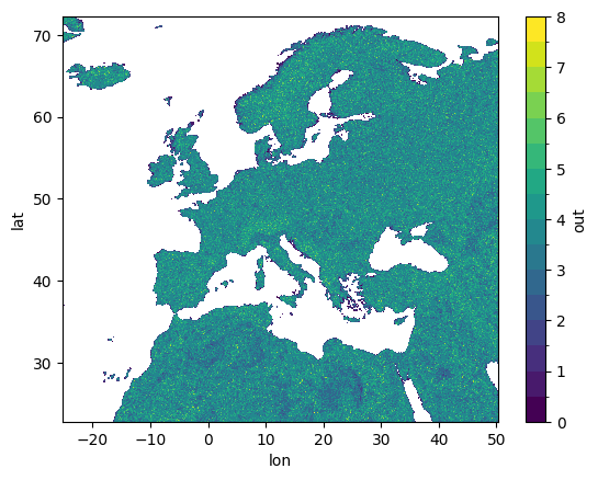
Below we show an example using move.downstream to find the number of gridcells draining to each point.
[ ]:
da = ekh.move.downstream(network, field, metric="sum")

da.plot.contourf(cmap="viridis", levels=20)
plt.show()